
You’ve spent weeks cleaning data and configuring your GPU cluster. You hit "start" on your Large Language Model pretraining run, only to watch the loss curve flatline or explode into NaNs. It’s a frustrating rite of passage for anyone training models at scale. But here’s the truth: most failures aren’t due to bad architecture or messy data. They’re caused by picking the wrong numbers for two specific knobs: learning rate and batch size.
If you are trying to figure out which settings actually move the needle, you’re in the right place. We’re cutting through the noise of thousands of possible configurations to focus on what truly matters in 2026. This isn’t just theory; it’s about saving you from burning $10,000 worth of GPU hours on a model that never converges.
The Two Kings of Hyperparameters
Let’s be honest: there are dozens of hyperparameters you could tweak. Weight decay? Sure. Dropout? Maybe. But if you have limited compute, ignore them all except two. Research consistently shows that learning rate and batch size account for roughly 70% of the variance in your final model performance. Everything else is secondary noise until these two are dialed in.
Why these two? Because they control the fundamental dynamics of how your model learns. The learning rate dictates the size of the steps your optimizer takes toward the minimum loss. Too big, and you overshoot, bouncing around wildly or diverging completely. Too small, and you crawl toward convergence so slowly that your budget runs out before you get anywhere useful. Batch size determines how many samples you look at before updating those weights. It affects gradient stability and computational efficiency. Get this balance wrong, and you either waste memory or introduce too much noise into your updates.
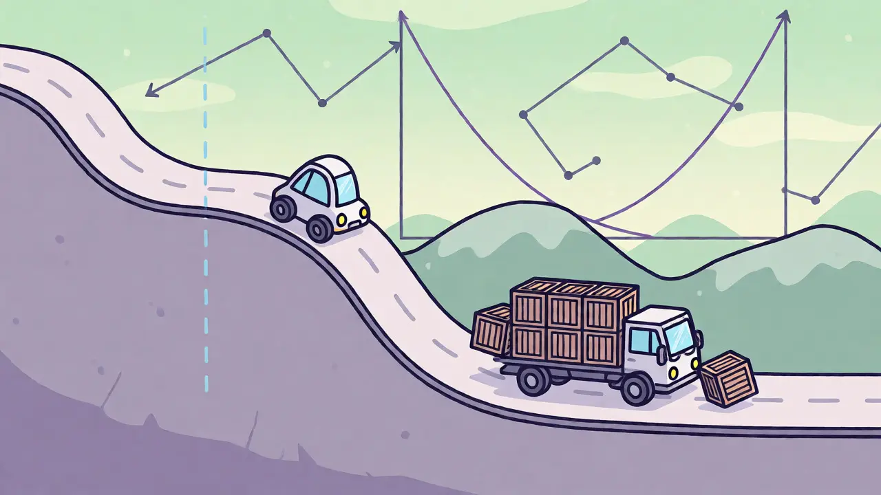
Think of it like driving a car. Learning rate is how hard you press the gas pedal. Batch size is how often you check your speedometer. If you floor the gas without checking your speed, you’ll crash. If you check the speedometer but barely touch the gas, you’ll never get there.
Scaling Laws Are No Longer Optional
A few years ago, finding the right hyperparameters meant brute-force grid searches-trying hundreds of combinations and hoping one worked. That approach is dead. It’s too expensive and too slow for modern models. Today, we rely on scaling laws empirical formulas that predict optimal hyperparameters based on model size and dataset volume.
The most robust framework currently available is known as the "Step Law," derived from massive experiments involving millions of GPU hours. It establishes clear power-law relationships. For example, the optimal learning rate doesn’t stay constant as your model grows. Instead, it scales down slightly as the number of parameters increases, but scales up slightly as your dataset gets larger. Specifically, the relationship follows a pattern where learning rate ($\eta$) is proportional to $N^{-0.11} \times D^{0.05}$, where $N$ is the number of parameters and $D$ is the dataset size in tokens.
This might sound abstract, but it has huge practical implications. If you double your dataset size, you don’t need to drastically change your learning rate. But if you increase your model size from 7 billion to 70 billion parameters, you must lower your peak learning rate to maintain stability. Ignoring this scaling behavior is why many practitioners see their large models fail while their smaller prototypes succeeded.
| Model Size (Parameters) | Dataset Size (Tokens) | Recommended Peak LR | Recommended Batch Size |
|---|---|---|---|
| 1B - 3B | 100B | ~3e-4 | ~2k - 4k tokens |
| 7B | 1T | ~2e-4 | ~8k tokens |
| 70B | 2T+ | ~1e-4 | ~16k+ tokens |
Note: These values are starting points based on standard transformer architectures. Always validate with short pilot runs.
The Convergence Cliff and Learning Rate Schedules
Here’s a trap that catches even experienced engineers: the "convergence cliff." Studies show that deviating from the optimal learning rate by just 5-10% can significantly degrade performance. Exceeding the optimal rate by more than 10% often leads to immediate instability, where gradients explode and training fails within the first few thousand steps.
But setting the peak learning rate is only half the battle. How you decay it over time matters just as much. Traditional schedules, like cosine annealing, often drop the learning rate to near zero by the end of training. Recent findings suggest this is suboptimal. Setting a fixed minimum learning rate (min_lr) rather than decaying to zero can reduce final loss by 12-18%. Why? Because a non-zero learning rate allows the model to continue escaping shallow local minima late in training, leading to better generalization.
Don’t just set `lr=3e-4` and walk away. Define a schedule that starts high, warms up gradually (to avoid early instability), and then decays to a sensible floor, not zero. A common mistake is using a warmup period that is too long, wasting valuable training steps at a low effective learning rate.
Batch Size: Stability vs. Speed
Batch size is tricky because it interacts with hardware constraints. Larger batches provide more stable gradient estimates, allowing for higher learning rates. However, they require more VRAM and can lead to worse generalization if not paired with appropriate regularization. The Step Law suggests that optimal batch size scales primarily with dataset size, following $B \propto D^{0.75}$.
This means that as you train on more data, you should generally increase your batch size. But here’s the catch: you can’t always do that physically. If you’re hitting memory limits, you might use gradient accumulation to simulate a larger batch size. Just remember that gradient accumulation is slower per step than true large-batch training. If you’re forced to use small physical batches, you may need to adjust your learning rate downward to compensate for the increased gradient noise.
Also, consider your architecture. Mixture-of-Experts (MoE) models behave differently than dense transformers. In MoE setups, the optimal learning rate can vary by up to 37% depending on the sparsity ratio of the experts. If you’re experimenting with MoE, treat the sparsity level as a key variable in your hyperparameter search.
Beyond the Big Two: What Else Matters?
Once your learning rate and batch size are solid, other parameters start to matter. Weight decay helps prevent overfitting, especially in large models trained on limited data. Typical values range from 0.01 to 0.1. Too high, and you underfit; too low, and you risk memorizing noise.
Warmup steps are critical for stability. Without a warmup phase, the initial updates can be too aggressive, causing divergence. A good rule of thumb is to set warmup steps to 1-5% of your total training steps. This gives the optimizer time to stabilize its momentum estimates before taking full-sized steps.
And don’t forget model depth. While not a tunable hyperparameter in the same way, the number of layers acts as a meta-hyperparameter. Deeper models require careful initialization and sometimes different learning rate schedules compared to wider, shallower models. Each additional layer adds complexity to the gradient flow, making deep networks more prone to vanishing or exploding gradients if not handled correctly.
Practical Workflow for 2026
So, how do you apply this tomorrow morning? Don’t start with a full-scale run. Follow this checklist:
- Estimate Optimal Values: Use current scaling law calculators or libraries like Optuna 4.2 (which now supports Step Law integration) to get baseline predictions for LR and batch size based on your N and D.
- Run a Pilot: Train for 1-2% of total steps. Monitor the loss curve closely. Is it smooth? Is it diverging?
- Adjust Based on Feedback: If loss explodes, lower LR by 20%. If loss plateaus early, increase LR or decrease batch size. If it’s noisy, increase batch size or add weight decay.
- Verify with a Grid: Once you have a stable configuration, run a small 3-point grid (optimal ±15%) to fine-tune. This usually takes less than 2,000 GPU hours for a mid-sized model.
- Document Everything: With EU AI Office guidelines requiring documentation for models over 10B parameters, keep detailed logs of your choices and outcomes. This aids reproducibility and future tuning.
Automated tools are getting better. LLM-assisted hyperparameter optimization can now outperform random search by 12-18% with constrained budgets. But human intuition still plays a role, especially when dealing with domain-specific data where scaling laws might deviate by 15-25%.
Common Pitfalls to Avoid
First, don’t assume that what worked for GPT-3 works for your custom dataset. Data distribution matters. Code-heavy corpora might prefer different learning rates than multilingual text. Second, beware of the "vanity metric" trap. Lower training loss doesn’t always mean a better model. Validate on held-out sets regularly.
Third, don’t neglect hardware compatibility. Some mixed-precision formats (like BF16 vs FP16) affect numerical stability, which in turn affects optimal learning rates. BF16 is generally more stable for large models, allowing for slightly higher learning rates than FP16 without risking overflow.
Finally, stop trying to optimize everything at once. Fix the big two, then move to the next tier. Trying to tune dropout, weight decay, and learning rate simultaneously is a recipe for confusion and wasted compute.
Do I really need to follow scaling laws for small models?
For very small models (under 1B parameters), scaling laws are less critical because the cost of failure is low. You can afford to grid search. However, for models above 1B parameters, the computational cost makes trial-and-error prohibitively expensive, so relying on predicted optima saves significant time and money.
What happens if my batch size is too small?
A too-small batch size introduces high variance in gradient estimates. This creates noisy updates, which can prevent the model from converging smoothly. You might need to lower your learning rate to compensate for this noise, which slows down training overall. It also reduces hardware utilization efficiency.
Is cosine decay still the best learning rate schedule?
Cosine decay is popular, but recent research suggests it’s not always optimal. Fixed minimum learning rates (where LR decays to a non-zero value) often yield better final perplexity scores, especially for large models. Experiment with linear decay to a floor versus cosine to zero to see which fits your specific task.
How does Mixture-of-Experts (MoE) change hyperparameter selection?
MoE models are sensitive to expert sparsity. The optimal learning rate can shift significantly based on how many experts are active per token. Dense models have more predictable scaling behaviors. For MoE, you often need to adjust learning rates downward if sparsity is high to maintain stability across different expert pathways.
Can I automate hyperparameter tuning entirely?
Not yet fully. While tools like Optuna and LLM-based optimizers help, they still require human oversight for setup and interpretation. Fully automated systems are emerging, but for complex, domain-specific tasks, human expertise in interpreting loss curves and adjusting strategies remains vital.