For years, building a better Large Language Model is an AI system trained on massive datasets to understand and generate human-like text felt like throwing money at a black box. You’d spin up thousands of GPUs, feed them petabytes of data, and hope the result was smarter than the last version. But that guesswork ended with the discovery of Neural Scaling Laws are empirical formulas that predict how model performance improves as you increase compute, parameters, or data size. These mathematical rules allow researchers to train tiny, cheap models and accurately predict how a billion-dollar supermodel will perform before writing a single line of training code for it.
This isn't just theory; it’s the engine behind every major AI breakthrough since 2020. Understanding these laws explains why some models fail despite huge budgets and why others punch above their weight class. It also reveals a shifting landscape where simply adding more parameters is no longer the only path to intelligence.
The Core Formula: C, N, and D
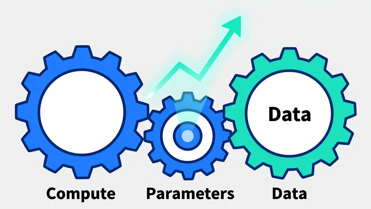
To understand neural scaling, you need to look at three variables. Researchers have found that language modeling performance-usually measured by "loss," which is essentially the error rate when predicting the next word-follows a predictable power law based on:
- C (Compute): The total amount of calculation power used during pretraining, often measured in floating-point operations (FLOPs).
- N (Parameters): The size of the artificial neural network, counted in billions of weights.
- D (Data): The size of the pretraining dataset, measured in tokens (chunks of text).
The basic insight is simple: if you plot these factors on a logarithmic scale, performance improves in a straight line. This means doubling your compute doesn’t double your quality, but it does improve it by a consistent, calculable percentage. Before this was proven, teams would tweak hyperparameters randomly. Now, they fit a curve to small experiments and extrapolate. If a 1-billion-parameter model shows a specific loss curve, the math tells you exactly what a 100-billion-parameter model should achieve under the same conditions.
This predictability changed everything. It turned AI development from an art into an engineering discipline. Companies could plan their infrastructure needs months in advance, knowing precisely how much GPU time they needed to hit a target performance level.
The GPT-3 Era: Bigger Was Better
When OpenAI released GPT-3 is a 175-billion-parameter transformer model released in 2020 that demonstrated significant few-shot learning capabilities, it seemed to confirm one thing: size matters most. GPT-3 was over 100 times larger than its predecessor, GPT-2. It didn’t just get slightly better; it started doing things smaller models couldn’t do at all, like answering complex questions without explicit fine-tuning.
At the time, the prevailing wisdom among many labs was to maximize N (parameters) as fast as possible. If you had extra compute, buy more GPUs to make the model bigger. Don’t worry about data quality or quantity as much; just scale the architecture. This approach worked well enough to push state-of-the-art results across dozens of benchmarks. Larger models made better use of the context window, remembering earlier parts of a conversation more effectively than their smaller cousins.
However, this strategy had a hidden cost. Many subsequent models, such as the 530-billion-parameter MT-NLG, were built on datasets similar in size to GPT-3’s. They were massive engines running on relatively little fuel. While they performed well, they weren’t reaching their theoretical potential because they ran out of data long before they ran out of capacity.
The Chinchilla Correction: Optimal Compute Allocation
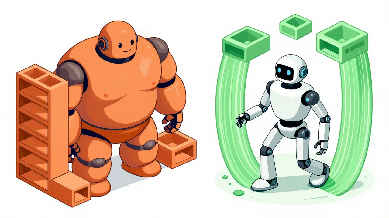
In 2022, DeepMind published a paper that shook the industry: Chinchilla Scaling Law is a set of guidelines determining the optimal ratio between model size and dataset size for a given amount of compute. The team trained a 70-billion-parameter model called Chinchilla. Despite being four times smaller than their previous flagship, Gopher (which had 280 billion parameters), Chinchilla performed better on nearly every benchmark.
Why? Because they changed the balance. Instead of dumping all their compute into making the model wider and deeper, they spent half of it collecting and cleaning more high-quality data. The Chinchilla law suggests that for every parameter you add, you should also increase the dataset size proportionally. Specifically, the optimal relationship is roughly linear: if you double the compute, you should double both the number of parameters AND the number of training tokens.
| Strategy | Focus | Data Usage | Efficiency Outcome |
|---|---|---|---|
| Pre-Chinchilla (e.g., Gopher) | Maximize Parameters (N) | Fixed/Limited Dataset | Suboptimal; model memorizes rather than generalizes |
| Chinchilla-Optimal | Balanced N and D | Scaled with Compute | Higher performance per FLOP; better generalization |
This finding forced a reckoning. Many existing models were "compute-suboptimal." They were too big for the data they saw. The fix wasn’t always to build bigger models, but to curate better, larger datasets. This shifted resources away from pure hardware expansion toward data engineering, cleaning pipelines, and copyright-compliant content acquisition.
Beyond Pretraining: The Rise of Inference-Time Compute
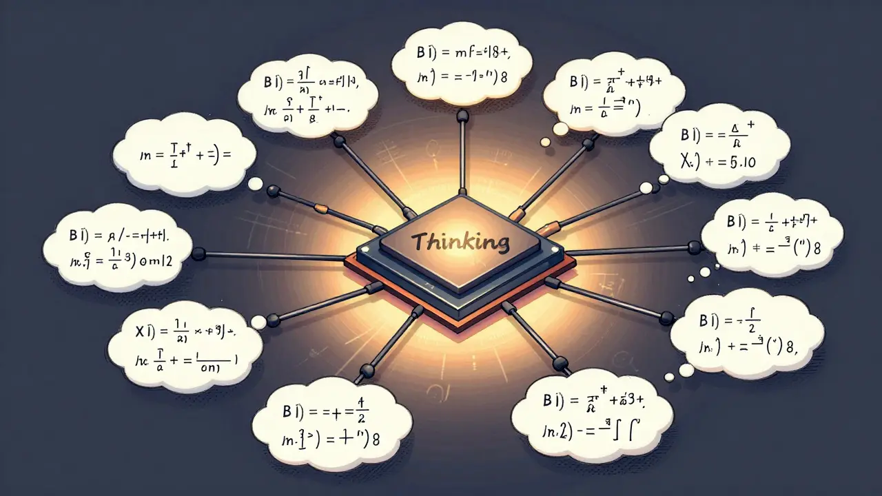
If scaling laws were static, we’d be done. But AI evolves. Recently, a new paradigm has emerged that challenges the traditional view that all intelligence must be baked in during pretraining. Models like OpenAI o1 is a reasoning-focused model that uses chain-of-thought processes to solve complex problems step-by-step and o3 are advanced reasoning models that allocate significant computational resources during the inference phase demonstrate that you can trade speed for accuracy.
Traditional scaling laws focus on pretraining compute. But these new "reasoning" models show that performance continues to scale if you invest compute at inference time. When faced with a hard math problem or a coding challenge, these models don’t just guess the answer. They generate long chains of thought, exploring multiple paths, checking their work, and refining their logic before outputting a final response.
This creates a new dimension to the scaling equation. You can now improve performance by allowing the model to "think" longer. This is particularly useful for tasks requiring logical deduction, where the correct answer isn’t just a pattern match from training data but requires multi-step verification. It means that for certain applications, a smaller model with high inference-time compute might outperform a larger model that answers instantly.
Emergent Abilities and Scaling Breaks
One of the most fascinating aspects of neural scaling is the phenomenon of emergent abilities. For a long time, critics argued that larger models wouldn’t fundamentally change; they’d just be marginally better at the same tasks. Then, at specific scale thresholds, models suddenly started passing benchmarks they previously failed completely, such as solving arithmetic problems or following complex instruction sets.
These aren’t magic tricks. They’re the result of complex interactions within the transformer architecture. As the model grows, its internal representations become dense enough to support abstract reasoning structures that were impossible in smaller networks. However, these breaks in the scaling law make prediction harder. A smooth power law might suggest a model is 90% ready for a task, but it might actually be stuck at 10% until it crosses a critical size threshold.
Researchers are still studying these discontinuities. They complicate the clean lines drawn by early scaling laws. Yet, even with these bumps, the overall trend remains reliable enough for strategic planning. The key takeaway is that while marginal gains are predictable, qualitative leaps require crossing specific scale barriers.
Practical Implications for Developers and Organizations
So, what does this mean for you if you’re building AI products or strategies in 2026?
- Don’t Overbuild: If you have limited compute, follow the Chinchilla guidelines. A smaller model trained on high-quality, diverse data will often beat a larger model trained on noisy, repetitive data.
- Use Small Models for Planning: Before committing to a massive training run, train a suite of small models. Fit the scaling curves. Extrapolate the cost-performance trade-offs. This saves millions in wasted GPU hours.
- Consider Inference Costs: With the rise of reasoning models, factor in the cost of generation. A model that takes 10 seconds to answer might be more accurate, but is it viable for your user experience? Balance pretraining efficiency with inference latency.
- Data Quality is King: Since data size (D) is equally important to parameters (N), invest heavily in data curation. Deduplication, filtering low-quality text, and ensuring diversity directly impact the scaling exponent.
The era of blind scaling is over. We now know the map. The question isn’t whether bigger is better, but how to optimally distribute your resources across parameters, data, and inference time to achieve the specific capabilities you need.
What are neural scaling laws in simple terms?
Neural scaling laws are mathematical formulas that predict how well an AI model will perform based on how much computing power, data, and model size you use. They allow developers to test small, cheap versions of a model and accurately guess the performance of a massive, expensive version before building it.
What is the Chinchilla Scaling Law?
The Chinchilla Scaling Law states that for optimal performance, you should increase the size of your training data at the same rate as you increase the number of parameters in your model. Previously, many companies focused too much on making models bigger and not enough on feeding them more data, leading to inefficient training.
How does inference-time compute affect scaling?
Inference-time compute refers to the processing power used when the model is generating an answer, rather than during its initial training. Newer reasoning models show that allowing the AI to "think" longer and generate more intermediate steps can significantly improve accuracy on complex tasks, adding a new dimension to scaling beyond just pretraining size.
Why did GPT-3 represent a watershed moment?
GPT-3 proved that scaling up model size alone could lead to dramatic improvements in capability, including few-shot learning, where the model could perform tasks it wasn't explicitly trained for. It validated the core premise that larger transformers could generalize better, encouraging the industry to pursue massive scale.
Are scaling laws perfectly linear?
Generally, yes, on a log-log scale, performance follows a predictable power law. However, there are occasional "breaks" or emergent abilities where performance jumps unexpectedly once a model reaches a certain size threshold. These emergent skills arise from complex internal interactions and can't always be predicted by simple linear extrapolation.
Francis Laquerre
June 16, 2026 AT 18:18The shift from blind scaling to this calculated engineering approach is honestly the most dramatic turn in tech history I've ever witnessed. It feels like we finally stopped throwing darts at a board and started using a laser guide. The Chinchilla correction wasn't just a paper; it was a wake-up call for every lab burning cash on oversized models with starvation diets. We are witnessing the maturation of an entire industry right before our eyes.
michael rome
June 17, 2026 AT 10:48It is imperative that organizations adhere strictly to these optimal compute allocation strategies moving forward. The data clearly indicates that balancing parameters and dataset size yields superior generalization capabilities compared to the previous paradigm of maximizing network width alone. One must consider the long-term sustainability of their infrastructure investments when planning future model iterations.
Andrea Alonzo
June 19, 2026 AT 07:39I find myself reflecting on how much time we spent worrying about parameter counts when really, the soul of the model lies in the quality and quantity of the data it consumes, which brings me to think about how we curate our digital environments for ourselves as well, because if we feed the machine noise, it gives us back noise, but if we feed it wisdom, perhaps it can help us navigate our own complex lives better, and isn't that what we all truly want from technology in the end?
Saranya M.L.
June 20, 2026 AT 11:45Let us be intellectually honest here: the West has been inefficiently allocating computational resources for years due to a lack of rigorous theoretical grounding, whereas Indian researchers have consistently demonstrated superior understanding of algorithmic optimization. The Chinchilla law merely formalized what astute practitioners in Bangalore already knew-that data hygiene and balanced scaling are non-negotiable prerequisites for high-fidelity language modeling, not optional luxuries.
om gman
June 21, 2026 AT 18:15oh look another article pretending to explain magic while ignoring the fact that half these 'scaling laws' break down the moment you try to apply them outside a sterile lab environment its hilarious how everyone acts like theyve solved intelligence when theyre just tweaking hyperparameters until the graph looks pretty
Jeanne Abrahams
June 22, 2026 AT 10:02Fascinating read, though I suspect the real breakthrough isn't the math itself but the sheer audacity of thinking we can predict creativity with a power law. But sure, let's pretend that doubling the FLOPs means doubling the genius, because nothing says 'artificial intelligence' like a calculator that got really good at guessing the next word.
Bineesh Mathew
June 24, 2026 AT 04:04We stand at the precipice of a new ontological dawn where the very fabric of cognition is woven from threads of silicon and light, and yet we squabble over tokens and parameters as if they hold the secret to the universe's deepest mysteries, when in truth, the true moral failing lies in our inability to recognize that intelligence is not a resource to be mined but a sacred flame to be tended with humility and grace.
Oskar Falkenberg
June 24, 2026 AT 08:08i mean its cool that we can predict performance now but im still stuck trying to get my local model to run without crashing my pc so maybe save the billion dollar supermodel talk for folks who actually have access to those kind of gpus would be great thanks