Training a modern Large Language Model (LLM) is less like writing code and more like conducting a symphony with thousands of musicians who occasionally forget their sheet music. You have billions of parameters to update, terabytes of data to process, and hardware that costs more than most houses. If you get the compute planning wrong, you aren't just losing time; you are burning cash on idle GPUs while your team waits for a single bottleneck to clear.
We used to think scaling models was just about throwing more money at bigger chips. But as we move into 2026, the game has changed. It’s no longer just about raw power. It’s about precision. How do you allocate resources so every GPU is working? How do you schedule jobs so smaller teams don’t starve while big models hog the cluster? And how do you keep the memory from exploding when the context window grows?
This guide breaks down the three pillars of efficient LLM training infrastructure: smart GPU allocation through parallelism, intelligent job scheduling, and aggressive memory management via checkpointing. We will look at real-world mechanics, not just theory, to help you build a pipeline that actually scales.
The Art of GPU Allocation: Parallelism Strategies
When you start training a model, the first decision is how to split the work across your available GPUs. The naive approach is Data Parallelism. In this setup, every GPU holds a full copy of the model. Each card processes a different batch of data, and then they average out the gradients. This works great for small models or when you have plenty of VRAM per card. But once your model hits tens of billions of parameters, one GPU can’t even hold the weights, let alone the activations.
That’s where advanced parallelism comes in. You need to break the model itself apart.
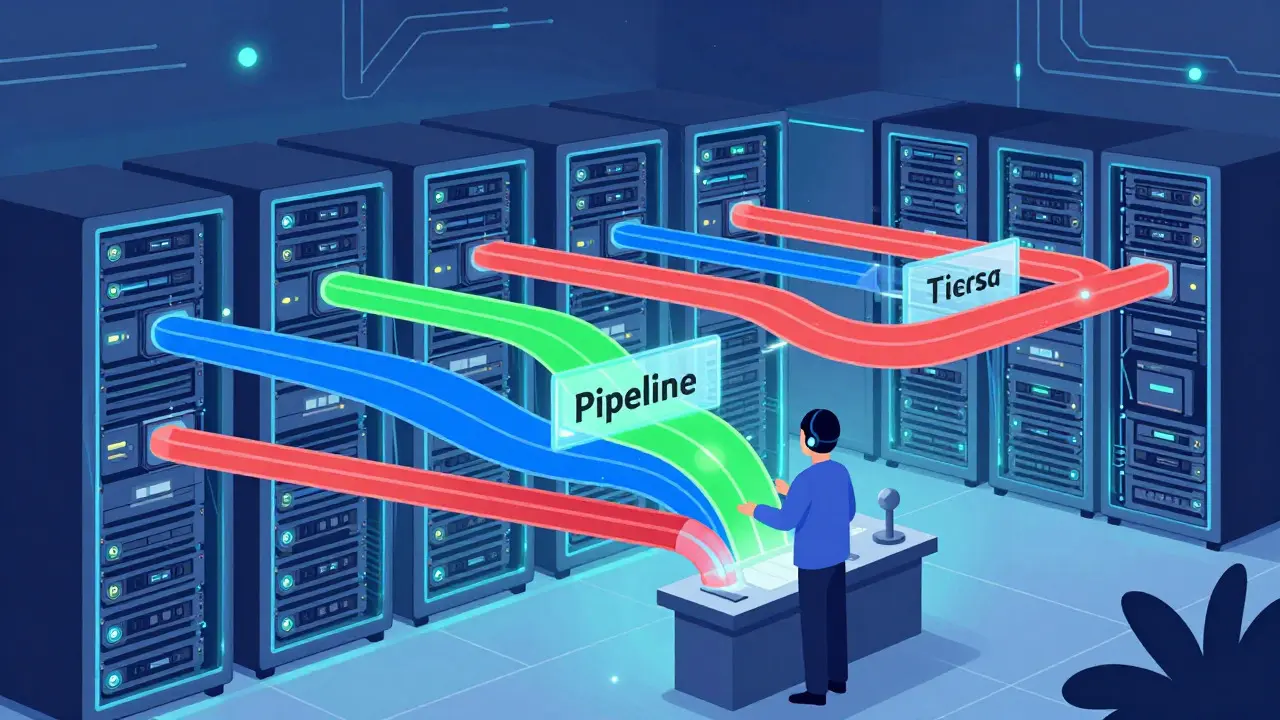
Pipeline Parallelism is a technique where the model is split into sequential stages, with each stage assigned to a different GPU or group of GPUs. Imagine an assembly line. GPU 1 handles the first few layers, passes the intermediate results to GPU 2, which handles the next set, and so on. The challenge here is "bubble" time-periods where some GPUs are waiting for others to finish. To fix this, frameworks use sophisticated scheduling algorithms like PipeDream or GPipe to keep the pipeline full. However, if your network bandwidth between nodes is slow, the communication overhead can eat up all your gains.
For even larger models, you need Tensor Parallelism is a method that splits individual matrix operations (tensors) across multiple GPUs within the same node. Instead of moving entire layers, you split the weight matrices themselves. This requires extremely fast interconnects, like NVIDIA NVLink, because the GPUs need to talk to each other during every forward and backward pass. If you’re using standard Ethernet or even InfiniBand without careful tuning, Tensor Parallelism can become a bottleneck rather than a booster.
A newer addition to the toolkit is Sequence Parallelism. As context windows grow to 128k or even 1 million tokens, the attention mechanism becomes a memory hog. Sequence Parallelism distributes the sequence length across GPUs. This is particularly useful for causal masking in autoregressive models. However, it introduces complexity. Not all parts of the transformer block benefit equally from sequence parallelism. You often see hybrid approaches, combining Tensor Parallelism for the attention heads and Sequence Parallelism for the MLP layers, to balance memory usage and computation speed.
| Strategy | Best For | Hardware Requirement | Key Challenge |
|---|---|---|---|
| Data Parallelism | Small to medium models | Standard PCIe/NVLink | Memory limits per GPU |
| Pipeline Parallelism | Very large models | InfiniBand/Ethernet | Bubble time/idle GPUs |
| Tensor Parallelism | Huge models (>10B params) | NVLink (High Bandwidth) | Communication overhead |
| Sequence Parallelism | Long context windows | NVLink/InfiniBand | Complex implementation |
Scheduling Mechanisms: Keeping the Cluster Busy
You have your parallelism strategy sorted. Now you face the reality of shared infrastructure. In most organizations, the GPU cluster is a multi-tenant environment. One team is pre-training a foundational model, another is fine-tuning for customer service, and a third is running inference tests. If you let them fight over resources, utilization drops, and costs skyrocket.
Traditional schedulers treat all GPUs as identical boxes. They are not. A cluster might have a mix of older H100s, newer Blackwell chips, and maybe some legacy V100s hanging around for legacy tasks. This is where heterogeneous-aware schedulers come in. Tools like Gavel or Gandivafair analyze the specific needs of a job. If a job is memory-bound, it gets routed to cards with higher VRAM. If it’s compute-bound, it goes to the fastest cores. This prevents a situation where a light workload sits on a massive GPU while a heavy task queues up behind it.
Another critical feature is Job Packing. Often, a single job doesn’t need an entire node. Maybe it only needs two GPUs. Without packing, those other six GPUs sit idle. Schedulers like Lucid or FGD allow multiple smaller jobs to share a single physical node, provided they don’t exceed the memory or compute limits. This is similar to container orchestration in Kubernetes but optimized for the unique demands of deep learning workloads.
Consider the scenario of hyperparameter tuning. You might want to test 50 different learning rates. Running these sequentially would take weeks. With proper scheduling, you can launch these as independent, short-lived jobs that fill in the gaps between larger training runs. Some advanced systems even use surrogate models-smaller, faster versions of your target model-to quickly evaluate configurations before committing expensive compute resources to the full-scale run.
Checkpointing and Memory Optimization
Memory is the silent killer of LLM training. Even if you have enough VRAM to hold the model weights, the activations generated during the forward pass can consume several times that amount. When you run out of memory, the job crashes. Restarting from scratch after three days of training is a nightmare.
This is where Gradient Checkpointing, also known as Activation Recomputation, saves the day. During the forward pass, instead of storing every intermediate activation in memory, the system stores only a subset. When the backward pass begins, it recalculates the missing activations on the fly. This trades computation for memory. You use more FLOPs, but you free up significant VRAM. For many teams, this is the difference between fitting a model on four GPUs or needing eight.
But what about saving progress? Checkpointing isn’t just about memory; it’s about durability. You need to save the state of your model periodically. The challenge is speed. Writing terabytes of model weights to disk every few steps can stall the training loop. Modern frameworks use asynchronous checkpointing, where the write operation happens in the background while the GPUs continue computing. They also employ compression techniques to reduce the size of the saved files without losing precision.
There’s also the strategic aspect of checkpointing. Research suggests that including intermediate checkpoints helps validate scaling laws. By monitoring loss curves at various stages, you can predict whether a model is on track to meet performance targets. If the early training data (the first 10 billion tokens) shows noisy convergence, you might decide to discard it and restart with a cleaner dataset. Having frequent, lightweight checkpoints makes this pivot possible without wasting weeks of compute.

Offloading Strategies: When VRAM Isn't Enough
Sometimes, even with parallelism and checkpointing, you hit a wall. The model is simply too big for the available GPU memory. Before buying more hardware, consider offloading.
CPU Offloading moves parts of the model or the optimizer states to the CPU’s RAM. CPU memory is cheaper and much larger than VRAM, though slower to access. Static offloading pre-assigns specific tensors to the CPU, while dynamic offloading adjusts in real-time based on memory pressure. Dynamic methods are smarter but add complexity to the scheduler.
If CPU RAM isn’t enough, you can go further to SSD Offloading. This allows you to train models that exceed the total memory of your entire machine by swapping data to disk. The performance penalty is significant-SSDs are orders of magnitude slower than VRAM-but it enables experimentation with massive models on modest hardware. This is particularly useful for research phases or when testing architecture changes before committing to a full-scale training run on premium clusters.
Fine-Tuning Efficiency: LoRA and Beyond
Not every project requires full pre-training. Most applications involve fine-tuning a pre-trained model like LLaMA or Mistral. Full fine-tuning updates all parameters, which is expensive. Parameter-Efficient Fine-Tuning (PEFT) methods change this calculus.
LoRA (Low-Rank Adaptation) is a technique that freezes the pre-trained model weights and injects trainable rank decomposition matrices into each layer. Instead of updating billions of parameters, you update a tiny fraction-often reducing trainable parameters by 10,000 times. This means you can fine-tune a 70-billion parameter model on a single consumer-grade GPU. The computational savings are immense, and the resulting adapters can be swapped easily to create different specialized models from the same base.
Other methods include Prefix Tuning, which adds a continuous vector to the input, and Prompt Tuning, which optimizes the input prompt itself. These techniques require minimal compute and are ideal for rapid iteration. When planning your compute, always ask: "Do I need to update the whole model, or can I use LoRA?" The answer usually dictates whether you need a cloud cluster or a local workstation.
Cost Reduction Through Distributed Training
One of the most counter-intuitive insights in recent years is that merging separate models can be cheaper than training one giant model. Amazon Science research showed that training separate models on different datasets and then merging them can reduce computational costs by up to 91%. This approach, sometimes called "mergeable models," allows you to parallelize the data distribution problem. Instead of shuffling diverse data through one model, you train specialized models on homogeneous data and combine them.
This changes how you plan your data pipeline. You no longer need a monolithic dataset. You can curate high-quality subsets for specific domains and merge them later. This also improves robustness. If one dataset has issues, it affects only one branch of the training, not the entire model. From a scheduling perspective, this means you can run multiple smaller, independent jobs that fit better into the gaps of your cluster schedule, rather than one massive job that blocks everything else.
Next Steps and Troubleshooting
As you design your compute plan, start with the constraints. How much VRAM do you have? What is your network bandwidth? Once you know the limits, choose your parallelism strategy. If you are memory-bound, prioritize Gradient Checkpointing and LoRA. If you are compute-bound, focus on Pipeline and Tensor Parallelism.
Monitor your Model FLOPs Utilization (MFU). If MFU is low, you likely have communication bottlenecks or bubble time in your pipeline. Adjust your parallelism degrees or optimize your data loader. Use profiling tools to identify where the time is spent. Is it in the forward pass? The backward pass? Or the synchronization steps?
Finally, automate your scheduling. Manual resource allocation doesn’t scale. Implement a scheduler that understands heterogeneity and supports job packing. This ensures that every dollar spent on hardware delivers maximum value. Remember, the goal isn’t just to train the model; it’s to train it efficiently, reliably, and cost-effectively.
What is the difference between Data Parallelism and Model Parallelism?
Data Parallelism replicates the entire model on each GPU, processing different batches of data simultaneously. It is simple but limited by the memory of a single GPU. Model Parallelism splits the model itself across multiple GPUs, allowing you to train models larger than any single GPU's memory. This includes Pipeline Parallelism (splitting layers) and Tensor Parallelism (splitting weights).
How does Gradient Checkpointing save memory?
Gradient Checkpointing reduces memory usage by not storing all intermediate activations during the forward pass. Instead, it stores only a subset and recomputes the rest during the backward pass. This trades additional computation time for significant VRAM savings, enabling larger batch sizes or deeper models.
When should I use LoRA instead of full fine-tuning?
Use LoRA when you have limited compute resources or want to fine-tune a very large model quickly. LoRA freezes the base model weights and trains small adapter modules, reducing trainable parameters by up to 10,000 times. It is ideal for domain adaptation or task-specific tuning without the cost of full fine-tuning.
What is the role of a heterogeneous-aware scheduler?
A heterogeneous-aware scheduler allocates jobs to GPUs based on their specific capabilities (e.g., memory size, compute speed). This prevents mismatches where a memory-heavy job is assigned to a low-memory GPU, improving overall cluster utilization and reducing wait times for users.
Can I train an LLM on a single consumer GPU?
Yes, for fine-tuning. Using techniques like LoRA and Gradient Checkpointing, you can fine-tune large models (e.g., 7B-13B parameters) on a single high-end consumer GPU (like an RTX 4090). Pre-training from scratch typically requires multiple enterprise-grade GPUs due to the sheer volume of data and parameters.