You’ve probably heard the term "Transformer" thrown around in every tech meeting, conference, or LinkedIn post since late 2017. But if you’re an engineer trying to actually build something with Generative AI, it can feel like a black box of matrix multiplications and attention heads. Why did this specific architecture replace everything that came before it? And more importantly, how do you tweak it without breaking your model?
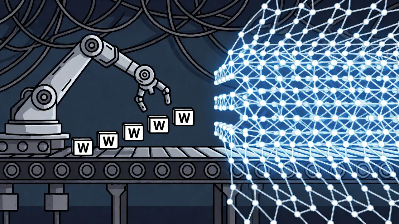
Here is the blunt truth: Transformers aren't magic. They are a clever rearrangement of linear algebra that solves the biggest bottleneck in sequential data processing-parallelism. Before Transformers, we relied on Recurrent Neural Networks (RNNs) that processed text one word at a time. This was slow and terrible at remembering context over long distances. The Transformer changed the game by looking at the entire sentence at once. This guide breaks down the mechanics, not just the theory, so you can debug your models and understand why your loss function isn't converging.
The Core Problem: Why RNNs Failed at Scale
To appreciate the Transformer, you have to understand what it replaced. Traditional sequence models like LSTMs and GRUs process inputs sequentially. If you want to predict the fifth word in a sentence, the model must first compute the state for words one through four. This creates two major issues for engineers:
- Sequential Bottleneck: You cannot parallelize training across time steps. GPUs love parallelism; RNNs hate it. This meant training large language models took weeks instead of days.
- Vanishing Gradients: As information travels from early tokens to later ones, the signal degrades. An LSTM might forget the subject of a sentence by the time it reaches the verb in a 50-word paragraph.
The Attention Mechanism solved both. By allowing every token to look at every other token simultaneously, the model captures long-range dependencies instantly. It doesn’t matter if the subject is at position 1 and the verb at position 100; the attention weight connects them directly.
Anatomy of a Transformer Block
A modern Large Language Model (LLM) is essentially a stack of identical blocks repeated dozens or hundreds of times. For example, GPT-3 has 96 layers. Each layer performs two main jobs: mixing information between tokens and processing each token independently. Let’s dissect the components you’ll encounter in PyTorch or TensorFlow implementations.
| Component | Function | Engineering Note |
|---|---|---|
| Token Embedding | Converts discrete tokens into continuous vectors. | Dimensions usually match the model size (e.g., 768 for BERT Base). |
| Positional Encoding | Adds order information to unordered embeddings. | Without this, "dog bites man" equals "man bites dog." |
| Multi-Head Self-Attention | Mixes context across all positions. | Splits vectors into multiple "heads" to learn different relationships. |
| Feed-Forward Network | Processes each token independently. | Usually expands dimensions by 4x then contracts back. |
| Layer Normalization | Stabilizes activations during training. | Critical for preventing exploding gradients in deep stacks. |
Demystifying Self-Attention
This is where most engineers get stuck. Self-attention sounds complex, but it’s just a weighted average. Imagine you are reading the sentence: "The animal didn't cross the street because it was too tired." When the model processes the word "it," it needs to know what "it" refers to. Self-attention calculates a score for every pair of words in the sentence.
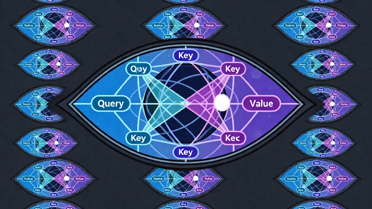
Mathematically, this involves three vectors derived from the input embedding: Query (Q), Key (K), and Value (V).
- Calculate Scores: Multiply Q and K^T. This tells you how much focus one word should pay to another.
- Scale: Divide by the square root of the key dimension. This prevents gradient explosions when dot products become large.
- Softmax: Convert scores into probabilities summing to 1. High probability means high relevance.
- Weighted Sum: Multiply these probabilities by V. The output is a new vector that blends information from relevant context.
Why "Multi-Head"? A single attention head might only capture syntactic structure. Multiple heads allow the model to attend to different types of relationships simultaneously-one head might track grammar, another coreference, and another sentiment. In practice, splitting the embedding dimension into smaller subspaces allows the model to project into different representation spaces before averaging the results.
Encoder vs. Decoder: Choosing Your Architecture
Not all Transformers are built the same way. The original paper described an Encoder-Decoder structure for translation. However, modern GenAI often uses only one half of this stack. Understanding which variant you are using dictates how you handle masking and generation.
Encoders (like BERT) use bidirectional attention. Every token sees every other token. This is perfect for understanding tasks like classification or search ranking because the full context is available immediately. There is no causal mask needed.
Decoders (like GPT) use causal masking. Token n can only see tokens 1 through n-1. This is essential for autoregressive generation-you can’t peek at the future while writing the next word. If you accidentally remove the causal mask in a decoder-only model, your training will be fast but your inference will be broken because the model cheats by seeing the answer during training.
Practical Implementation Pitfalls
When you move from paper to production, several engineering challenges emerge. Here are the most common traps I’ve seen in deployment scenarios.
1. Positional Encoding Choices
The original Transformer used fixed sinusoidal functions for positional encoding. Modern models often use learned positional embeddings or Rotary Positional Embeddings (RoPE). RoPE, used in Llama and Mistral, encodes relative positions rather than absolute ones. This helps with extrapolation-if you train on sequences of length 2048, RoPE makes it easier to handle length 4096 without retraining. If you are building a custom model, start with RoPE unless you have a specific reason not to.
2. Memory Management
Self-attention scales quadratically with sequence length ($O(n^2)$). Doubling the context window quadruples the memory usage for attention matrices. For an engineer deploying a model with a 100k context window, this is a massive VRAM hit. Techniques like Flash Attention optimize this by keeping intermediate calculations in SRAM rather than HBM, reducing memory overhead significantly. Always check if your library supports Flash Attention v2 before assuming standard implementation efficiency.
3. The Pre-training vs. Fine-tuning Gap
Transformers excel at transfer learning. You rarely train from scratch. Instead, you take a pre-trained checkpoint and fine-tune it. However, catastrophic forgetting is real. If you fine-tune a general-purpose model on a narrow dataset (like legal contracts), it may lose its ability to generate general English. Use techniques like Low-Rank Adaptation (LoRA) to freeze the main weights and train small adapter matrices. This preserves the base knowledge while adapting to your domain efficiently.
Scaling Laws and Performance Metrics
How big should your model be? Chinchilla scaling laws suggest that for optimal performance, you need roughly 20 tokens of training data per parameter. If you have 1 billion parameters, you need 20 billion tokens. Under-training a large model is worse than over-training a small one. Engineers often make the mistake of choosing a larger model size without ensuring they have enough diverse data to support it.
Evaluation metrics also differ from traditional ML. Perplexity measures how surprised the model is by the next token. Lower perplexity is better, but it doesn’t guarantee human-like quality. For generative tasks, human evaluation or automated benchmarks like HELM (Holistic Evaluation of Language Models) provide a more accurate picture of utility.
Future Trends: Beyond Text
The Transformer architecture is no longer just for NLP. Vision Transformers (ViT) treat images as sequences of patches, applying the same attention mechanisms. Multimodal models like CLIP connect text and image embeddings in the same space. As an engineer, expect to see Transformer blocks embedded in non-text domains, from protein folding (AlphaFold) to audio synthesis. The core principle-attending to relationships between elements regardless of modality-remains constant.
What is the difference between Multi-Head Attention and Single-Head Attention?
Single-head attention computes one set of Query, Key, and Value projections. Multi-head attention splits the embedding dimension into multiple smaller subspaces, performing attention in parallel for each subspace, and then concatenating the results. This allows the model to jointly attend to information from different representation subspaces at different positions, capturing diverse linguistic features like syntax, semantics, and coreference simultaneously.
Why do Transformers require positional encoding?
Unlike RNNs, Transformers process all tokens in parallel and have no inherent notion of order. Without positional encoding, the model would treat the input as a bag of words, unable to distinguish between "dog bites man" and "man bites dog." Positional encodings inject order information into the token embeddings, either through fixed mathematical functions (sinusoidal) or learned parameters.
Can I use a Transformer for tabular data?
Yes, architectures like TabTransformer adapt the standard Transformer block for tabular data. They apply self-attention to categorical features to capture interactions between columns, while numerical features are often processed separately. While XGBoost still dominates many tabular tasks, Transformers offer advantages when feature interactions are complex and numerous.
What is the computational complexity of self-attention?
Standard self-attention has a time and space complexity of $O(n^2)$, where $n$ is the sequence length. This means doubling the sequence length quadruples the computational cost. This quadratic scaling is the primary bottleneck for very long contexts, leading to the development of efficient attention variants like Linear Attention or Sparse Attention.
Do I need to normalize inputs before feeding them into a Transformer?
Typically, no. Transformers use Layer Normalization internally within each block to stabilize activations. Inputs are usually tokenized and embedded directly. Unlike CNNs which benefit from pixel normalization, Transformers rely on their internal normalization layers and residual connections to manage scale variations across deep networks.